
 Force Field X
Thermodynamic NPT Organic Crystal Polymorph Search
The majority of polymorph search algorithms are based on searching a potential energy surface over space groups, unit cell parameters and molecular coordinates. Here we present a novel thermodynamic search procedure1 that samples the phase space of polymorphs at a prescribed temperature and pressure (i.e. NPT).
The general procedure for the thermodynamic polymorph search is as follows:
- Prepare space groups with random starting coordinates.
- Setup and run a Thermodynamics command.
Preparation of Space Group Simulation Directories
To perform the polymorph search in each target space group, a input coordinate file in XYZ (or PDB) format is needed. In this example, we are using carbamazepine (CBZ).
                    30 CBZ.xyz
                    1 O 1.056327 2.681279 -1.205416 415 14
                    2 N 0.013517 0.882342 -0.199472 407 4 5 14
                    3 N -1.208192 2.632570 -1.309045 409 14 29 30
                    4 C 1.239504 0.196002 0.163542 402 2 6 10
                    5 C -1.188951 0.163264 0.185422 402 2 7 11
                    6 C 1.574003 -1.017457 -0.500887 406 4 8 12
                    7 C -1.513347 -1.052206 -0.479181 406 5 9 13
                    8 C 0.707998 -1.587940 -1.539462 404 6 9 19
                    9 C -0.651244 -1.601238 -1.531369 404 7 8 20
                    10 C 2.078718 0.718406 1.168788 408 4 15 21
                    11 C -2.003096 0.649430 1.228952 408 5 16 22
                    12 C 2.765145 -1.677153 -0.111878 403 6 17 23
                    13 C -2.689226 -1.732175 -0.079161 403 7 18 24
                    14 C 0.015450 2.092212 -0.925575 401 1 2 3
                    15 C 3.252341 0.045038 1.527667 405 10 17 25
                    16 C -3.159986 -0.045033 1.601550 405 11 18 26
                    17 C 3.597157 -1.157107 0.884816 410 12 15 27
                    18 C -3.505835 -1.238789 0.943487 410 13 16 28
                    19 H 1.213457 -2.006500 -2.410769 414 8
                    20 H -1.157318 -2.032494 -2.396149 414 9
                    21 H 1.805364 1.654177 1.653179 412 10
                    22 H -1.722357 1.572906 1.732896 412 11
                    23 H 3.038054 -2.613634 -0.600567 417 12
                    24 H -2.954555 -2.669119 -0.570959 417 13
                    25 H 3.896980 0.457503 2.301469 416 15
                    26 H -3.786286 0.338775 2.404700 416 16
                    27 H 4.508661 -1.683532 1.163694 413 17
                    28 H -4.401250 -1.784798 1.236556 413 18
                    29 H -1.190268 3.504894 -1.820183 411 3
                    30 H -2.085532 2.148253 -1.167517 411 3
The property file (analogous to a TINKER keyword file) specifies the space group, (starting) unit cell information, and AMOEBA parameters for the molecule. The latter can be generated using the PolType 22,3 program developed in the lab of Professor Pengyu Ren (in this case carbamazepine AMOEBA parameters are contained in CBZ.patch). It is important to specify a space group (e.g. P1) and unit cell parameters so that the FFX PrepareSpaceGroups command recognizes the system as respecting periodic boundary conditions.
                    forcefield AMOEBA_BIO_2018
                    patch /ABSOLUTE/PATH/TO/CBZ.patch
                    spacegroup P1
                    a-axis 10.0
                    b-axis 10.0
                    c-axis 10.0
                    alpha 90.0
                    beta 90.0
                    gamma 90.0
                    heavy-hydrogen true
FFX handles the creation of space groups through the PrepareSpaceGroups command seen below. For the purpose of this example, we will search for known carbamazepine polymorphs archived at the Cambridge Crystallography Data Centre (CCDC). First, we will search in the space group P21/c (CBMZPN01). Other helpful flags can be identified for the creation of space groups by using the following command: ffxc PrepareSpaceGroups -h.
ffxc PrepareSpaceGroups --sg=P21/c CBZ.xyzEach of the space groups identified by the PrepareSpaceGroups command should now have their own subdirectories. Each subdirectory contains a space group specific property file and coordinate file. As long as an absolute path to the patch file (i.e., CBZ.patch) file was given, no further files are needed in each space group subdirectory.
Thermodynamic Polymorph Search for a Space Group
The Thermodynamics command is used to perform a polymorph search in each space group. The algorithm operates in the NPT ensemble, and alchemically modulates intermolecular interactions using a lambda (L) state variable. At L=0, all intermolecular interactions are zero (i.e. vacuum), while at L=1, all intermolecular interactions (including between space group symmetry mates) are full strength (i.e. crystalline). The Orthogonal Space Random Walk algorithm is used to sample the thermodynamic path between vacuum and crystalline end states, including fully flexible sampling of atomic coordinates and unit cell parameters fluctuations under control of a Monte Carlo barostat. Hundreds to thousands of transitions between the vacuum and crystalline phases for the specified molecule are simualted. 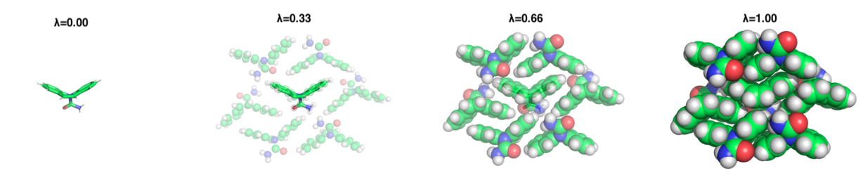 The above image depicts the alchemical thermodynamic path traversed during a simulation. Both ends of the lambda path are physical states, with 0 defining a molecule in vacuum and 1 defining the crystalline state, while intermediate lambda values are alchemical.
ffxc Thermodynamics -Dlambda-bin-width=0.02 -Dost-opt-energy-window=10.0 -Dpolarization=none --iW
                    --minD=1.1 -d 2.0 -r 0.1 -w 10.0 -l 0.0 -n 1000000 -Q 0 -i stochastic --rsym 2.0 --ruc
                    1.25 -t 298.5 --ac ALL -p 1.0 --bM=0.0001 -o CBZ.xyz
| Flag | Description |
|---|---|
| -Dmdmove-full=true | Utilizes orthagonal space tempering algorithm for Monte Carlo molecular dynamics. |
| -Dlambda-bin-width=0.02 | Determines the amount of change in the state variable lambda. |
| -Dost-opt-energy-window=10.0 | Structures within 10.0 kcal/mol of the minimum energy will be saved. |
| -Dpolarization=none | Determines behavior for atomic polarizability (NONE, DIRECT, or MUTUAL). |
| --iW | Enforces that each walker maintains its own histogram (i.e., independent). |
| --minD=1.1 | Specify the minimum allowable density to be 1.1 (g/cc). |
| -d 2.0 | Time step in femtoseconds (2 assumes use of the heavy-hydrogen property). |
| -r 1.0 | Interval to report thermodynamics (psec). |
| -w 10.0 | Interval to write coordinate snapshots (psec). |
| -l 0.0 | Initial lambda value (L=0 specifies vacuum in this case). |
| -n 1000000 | Number of MD steps. |
| -Q 0 | Number of equilibration steps before evaluation of thermodynamics. |
| -i stochastic | Specify the stochastic dynamics integrator. |
| --rsym 2.0 | Apply a random Cartesian symmetry operator with a random translation in the range -X .. X; less than 0 disables. |
| --ruc 1.25 | Apply random unit cell axes to achieve the specified density (g/cc). |
| -t 298.15 | Temperature (kelvin). |
| --ac ALL | Specify alchemical atoms for simulation. |
| -p 1.0 | Specify use of a MC Barostat at the given pressure (atm); the default 0 disables NPT and will not search unit cell parameters (only atomic coordinates). |
| --bM 0.0032 | Specify the OST Gaussian bias magnitude (kcal/mol). |
| -o | Optimize and save low-energy snapshots. |
The successful use of this setup for the Thermodynamics command will produce multiple optimized coordinate files with unit cell parameters contained in the second line (i.e. CBZ_opt.xyz_#). These files can be concatenated together into an archive file (i.e. CBZ.arc). Although each optimized file is a proposed polymorph for the specified molecule, those with the lowest potential energies and favorable densities are strongest candidates. Redundant structures can be found via tight minimization; those in the same energy well will optimize to similar potential energies. A minimization over coordinates and unit cell parameters can be performed using the following command:
ffxc MinimizeCrystals -ce 0.001 CBZ.arc| Flag | Description |
|---|---|
| -c | Alternate between optimization of coordinates and lattice parameters. |
| -e=0.001 | Specify convergence criteria (kcal/mol/A). |
At this point, a series of ab initio polymorphs for a desired molecule have been produced, limited by the quality of the AMOEBA force field parameters and/or convergence of the sampling.
Example Output and Analysis
Utilizing the input files and setup for the Thermodynamics command seen above should produce logging that alternates between the following:
                         Time      Kinetic    Potential        Total     Temp      CPU
                         psec     kcal/mol     kcal/mol     kcal/mol        K      sec
                                    7.9140     -11.4425      -3.5285   295.00
                    The free energy is      -2.2174 kcal/mol (Total Weight: 1.18e+05, Tempering: 0.9996, Counts:            0).
                    L=0.0000 (  0) F_LU=   -0.0000 F_LB=   -0.0001 F_L=   -0.0001 V_L=    0.0570
                    1.000e-01      14.7908      -5.3560       9.4348   551.33    4.895
                    L=0.0002 (  0) F_LU=   -0.0000 F_LB=   -0.0009 F_L=   -0.0009 V_L=    0.0873
                    2.000e-01       4.9389      -5.9505      -1.0116   184.10    2.345
                    The free energy is      -2.2174 kcal/mol (Total Weight: 1.18e+05, Tempering: 0.9996, Counts:           24).
                    L=0.0005 (  0) F_LU=   -0.0000 F_LB=   -0.0024 F_L=   -0.0024 V_L=    0.0998
                    3.000e-01       8.9068      -4.6493       4.2575   332.01    2.689
                    L=0.0013 (  0) F_LU=   -0.0000 F_LB=   -0.0065 F_L=   -0.0065 V_L=    0.0814
                    4.000e-01       8.0651      -6.6926       1.3725   300.63    2.314
                    The free energy is      -2.2174 kcal/mol (Total Weight: 1.18e+05, Tempering: 0.9996, Counts:           49).
                    L=0.0023 (  0) F_LU=   -0.0001 F_LB=   -0.0120 F_L=   -0.0121 V_L=    0.1067
                    L=0.0026 (  0) F_LU=   -0.0002 F_LB=   -0.0142 F_L=   -0.0143 V_L=   -0.0318
                    5.000e-01      11.0130      -6.7040       4.3090   410.51    2.749
                    L=0.0022 (  0) F_LU=   -0.0001 F_LB=   -0.0122 F_L=   -0.0123 V_L=   -0.0651
                    6.000e-01       7.0453      -1.7482       5.2970   262.62    2.302
                     .               .            .            .          .       .
                     .               .            .            .          .       .
                     .               .            .            .          .       .
                    8.400e+00       9.8824     -15.0173      -5.1349   368.37   29.656
                    L=0.9832 ( 49) F_LU=  -58.7961 F_LB=   66.6668 F_L=    7.8707 V_L=   -0.1075
                    8.500e+00       6.1456     -15.2336      -9.0880   229.08   18.744
                    L=0.9811 ( 49) F_LU=  -63.0950 F_LB=   66.7767 F_L=    3.6817 V_L=   -0.0536
                    The free energy is      -1.8853 kcal/mol (Total Weight: 1.21e+05, Tempering: 1.0000, Counts:         1024).
                    8.600e+00       7.4795     -12.4058      -4.9263   278.80   18.998
                    L=0.9801 ( 49) F_LU=  -58.8955 F_LB=   66.6010 F_L=    7.7055 V_L=   -0.0124
                    8.700e+00       9.6898     -11.6549      -1.9651   361.19   16.484
                    L=0.9809 ( 49) F_LU=  -68.7993 F_LB=   61.7536 F_L=   -7.0458 V_L=   -0.0155
                    8.800e+00       9.2525     -17.4102      -8.1578   344.89   18.014
                    The free energy is      -1.8854 kcal/mol (Total Weight: 1.21e+05, Tempering: 1.0000, Counts:         1049).
                    L=0.9802 ( 49) F_LU=  -64.6803 F_LB=   65.4695 F_L=    0.7893 V_L=   -0.0401
The above section monitors the advancement of the stochastic dynamics simulation with respect to time. "L" indicates the current lambda value and its discrete bin in parentheses. The lambda value evolve between zero (i.e. denoting no intermolecular interactions in vacuum) and one (i.e. the molecule is subject to full crystalline periodic boundary conditions in the defined space group).
- F_LU is the partial derivative of the potential energy with respect to lambda (i.e., 1-D bias).
- F_LB is the partial derivative of the orthogonal space bias with respect to lambda (i.e., 2-D bias).
- F_L is the sum of F_LU and F_LB (i.e., total bias).
- V_L is the velocity of the lambda particle.
The column labels at the top of this section correlate to the numeric rows that do not have alternative labels. The Density, unit cell parameters (UC: a b c alpha beta gamma), percentage of unit cell length moves accepted (MCS), and the percentage of unit cell angle moves accepted (MCA) are also listed in this section.
                    Weight   Lambda      dU/dL Bins  <dU/dL>    g(L)  f(L,<dU/dL>) Bias    dG(L) Bias+dG(L)
                    5.90e+02 0.00500    -1.0     1.0     0.00    -0.00     0.03     0.03     0.00       0.03
                    4.57e+02 0.02000    -1.0     1.0     0.00    -0.00     0.03     0.03     0.00       0.03
                    6.52e+02 0.04000    -1.0     1.0     0.00    -0.00     0.02     0.02     0.00       0.02
                    3.23e+02 0.06000    -1.0     1.0     0.00    -0.00     0.02     0.02     0.00       0.02
                    1.25e+02 0.08000    -1.0     1.0     0.00    -0.00     0.01     0.01     0.00       0.01
                    1.24e+02 0.10000    -1.0     1.0     0.00    -0.00     0.01     0.01     0.00       0.01
                    1.31e+02 0.12000    -1.0     1.0     0.00    -0.00     0.01     0.01     0.00       0.01
                    2.20e+02 0.14000    -1.0     1.0     0.00    -0.00     0.01     0.01     0.00       0.01
                    2.70e+02 0.16000    -1.0     1.0     0.00    -0.00     0.01     0.01     0.00       0.01
                    3.06e+02 0.18000    -1.0     1.0     0.00    -0.00     0.01     0.01     0.00       0.01
                    2.31e+02 0.20000    -1.0     1.0     0.00    -0.00     0.01     0.01     0.00       0.01
                    1.25e+02 0.22000    -1.0     1.0     0.00    -0.00     0.01     0.01     0.00       0.01
                    1.48e+02 0.24000    -1.0     3.0     1.00    -0.01     0.01    -0.00     0.02       0.02
                    8.70e+01 0.26000    -1.0     3.0     1.00    -0.03     0.01    -0.02     0.04       0.02
                    4.30e+01 0.28000    -1.0     3.0     1.00    -0.05     0.00    -0.05     0.06       0.01
                    6.60e+01 0.30000    -1.0     3.0     1.00    -0.07     0.00    -0.07     0.08       0.01
                    8.50e+01 0.32000    -1.0     7.0     3.00    -0.11     0.00    -0.11     0.14       0.03
                    4.40e+01 0.34000    -1.0     7.0     3.00    -0.17     0.00    -0.17     0.20       0.03
                    1.32e+02 0.36000    -1.0    13.0     6.00    -0.26     0.00    -0.26     0.32       0.06
                     .        .           .       .       .        .        .        .        .          .
                     .        .           .       .       .        .        .        .        .          .
                     .        .           .       .       .        .        .        .        .          .
                    3.12e+03 0.88000   -43.0     3.0   -20.29    -2.70     0.04    -2.66     2.50      -0.16
                    3.58e+03 0.90000   -49.0     5.0   -22.49    -2.28     0.04    -2.23     2.05      -0.18
                    5.22e+03 0.92000   -61.0     5.0   -28.89    -1.76     0.06    -1.71     1.47      -0.23
                    6.59e+03 0.94000   -71.0    -5.0   -39.91    -1.07     0.08    -0.99     0.67      -0.32
                    8.29e+03 0.96000   -77.0    -7.0   -45.94    -0.22     0.13    -0.09    -0.24      -0.33
                    1.27e+04 0.98000   -93.0   -11.0   -55.95     0.80     0.30     1.10    -1.36      -0.26
                    6.43e+04 0.99500  -107.0    -9.0   -60.32     1.67     0.42     2.08    -1.97       0.12
This section displays a summary of the orthogonal space histogram, which contains all information necessary to compute free energy differences.
- Weight is the integral of the bias added over all dU/dL bins at a fixed lambda.
- Lambda displays the mean lambda value for each lambda bin.
- dU/dL Bins display the min/max of the instantaneous dU/dL sampled for each lambda bin.
- <dU/dL> gives the thermodynamic average of dU/dL (i.e. the force used during thermodynamic integration).
- g(L) is the 1D orthogonal space bias for a given lambda.
- f(L,<dU/dL>) is the 2D bias evaluated at (lambda, <dU/dL>).
- Bias is the sum of the 1D and 2D bias columns.
- dG(L) is the free energy difference from L=0 to the current lambda bin.
- Bias+dG(L) is the sum of the Bias and dG(L) for the current lambda bin.
As a simulation converges, the sum Bias+dG(L) approaches a constant and a random walk along lambda results.
| Number of Molecules Compared | P21/c | Pbca | C2/c | H-3 |
|---|---|---|---|---|
| 15 | 0.440 | 0.202 | 0.372 | 0.308 |
| 32 | 0.545 | 0.209 | 0.415 | 0.342 |
| 40 | 0.620 | 0.210 | 0.433 | 0.352 |
The above table shows the RMSD deviations of FFX produced polymorphs, compared to those experimentally observed in the CCDC. These comparisons are done with increasing number of molecules. The starting files for each of the space groups can be found below.
| Space Group | Coordinate File | Property File | Parameter File |
|---|---|---|---|
| P21/c | CBZ_p21_c.xyz | CBZ_p21_c.properties | CBZ.patch |
| Pbca | CBZ_pbca.xyz | CBZ_pbca.properties | CBZ.patch |
| C2/c | CBZ_c2_c.xyz | CBZ_c2_c.properties | CBZ.patch |
| H-3 | CBZ_h-3.xyz | CBZ_h-3.properties | CBZ.patch |
Citation:
Nessler, Okada, Kinoshita, Nishimura, Nagata, Fukuzawa, Yonemochi, & Schnieders. (2024). Crystal Polymorph Search in the NPT Ensemble via a Deposition/Sublimation Alchemical Path. Cryst. Growth Des. DOI: 10.1021/acs.cgd.3c01358
References:
1. 34th Annual Meeting of the Academy of Pharmaceutical Science and Technology, June 16-18 2019, Toyama, Japan, Prospects for applying in-silico crystal structure prediction to drug development. Hiroomi Nagata*, Okimasa Okada*, Aaron Nessler**, and Michael Schnieders**.
Mitsubishi Tanabe Pharma Corporation*
The University of Iowa**
2. Wu, J. C., Chattree, G., Ren, P. (2012). Automation of AMOEBA polarizable force field parameterization for small molecules. Theoretical chemistry accounts, 131(3), 1138. https://doi.org/10.1007/s00214-012-1138-6
3. Walker, B., Liu, C., Wait, E., Ren, P. (2022). Automation of AMOEBA polarizable force field parameterization for small molecules: Poltype 2. J. Comput. Chem. 2022, 43( 23), 1530. https://doi.org/10.1002/jcc.26954